In univariate data analysis, the median is often used as an alternative to the mean because the mean is sensitive to outliers in the data, whereas the median is a robust statistic. For higher-dimensional data, the mean and the centroid are both used to represent the "center" of a cloud of high-dimensional points. However, these statistics, too, are sensitive to outliers.

One robust high-dimensional robust estimate of a center is the geometric median. Unfortunately, the geometric median is not simple to compute. You can compute the geometric median in SAS by using nonlinear optimization or iterative matrix computations. A simpler "center" is the medoid.

What is a medoid?

The medoid (pronounced MEH-doyd, which rhymes with "red void") is a robust statistic that is conceptually easy to understand. Given a set of points, X = {x₁, x₂, ..., x_k}, the medoid is a point, m, in the set that minimizes the sum of the distances from m to every other point in X. Notice from this definition that the medoid is always one of the data points. Because the medoid minimizes the distance to other points, the medoid can be used to represent the center of a high-dimensional point cloud. The medoid tends to be more robust to outliers than means or centroids.

Compute the medoid in SAS

Calculating the medoid is straightforward, but it requires calculating all pairwise distances. You first load the data into a matrix, X, that has n rows. You compute the matrix of pairwise distances by using the DISTANCE function in SAS IML (or by using PROC DISTANCE in Base SAS). The distance matrix is symmetric, so you can sum either the columns or the rows to find the sum of the distances. (I'll sum the rows.) If the k_th row has the smallest sum, the k_th point in the data is the medoid.

• Use the DISTANCE function in SAS IML to compute the full n x n distance matrix, D, where D[i, j] is the distance between row i and row j in the X matrix. By default, the DISTANCE function computes the Euclidean distance.
• Use the "summation" subscript reduction operator ([ ,+]) to sum across the columns of the distance matrix. The resulting vector, sumDist, holds the sum of the distances from each point i to all others.
• Use the "minimum index" subscript reduction operator ([>:<]) to find the index corresponding to the minimum value in the sumDist vector.

Compute the medoid in two dimensions

The following example uses 10 points in two dimensions. The computation shows that medoid is the point (7, 5), which is the nineth row of the matrix of points:

proc iml;
X = {7 3,
     8 7,
     4 9,
     9 6,
     8 4,
     5 8,
     8 5,
     3 7,
     7 5,   /* This is the 9th row */
     4 5};
 
/* The medoid (https://en.wikipedia.org/wiki/Medoid) is the data value (say, y=x[j]) that 
   minimizes the sum of the distances from y to every other point */
D = distance(X);           /* D[i,] is the distance from X[i,] to every other point */
sumDist = D[ ,+];          /* sum of distances from X[i,] to every other point */
rowIdx = sumDist[>:<];     /* row that has the smallest sum of distances */
medoid = X[rowIdx, ];      /* coordinates of the medoid */
 
print sumDist[r=(1:nrow(X))];
print medoid[r=rowIdx c={'x' 'y'}];

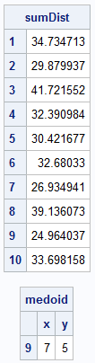
In this example, the sumDist vector contains the sum of the distances from each point to all others. The 9th point, with coordinates (7, 5), has the smallest total distance (24.96), so it is the medoid. You can use a scatter plot to visualize the data and the medoid:

/* visualize the data and the medoid */
title "Medoid in 2-D";
isMedoid = j(nrow(X), 1, 0);  /* binary indicator variable */
isMedoid[rowIdx] = 1;
call scatter(X[,1], X[,2]) group=isMedoid grid={x y} option="markerattrs=(symbol=CircleFilled size=12)";

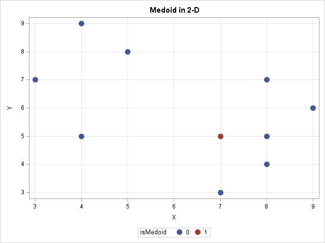
The point (7, 5) is displayed by using a red marker. The sum of the distances from (7, 5) to the other points is smaller than the sum of distances for any other point. From among the points, it is the best choice for the "center" of the point cloud.

Compute the medoid in higher dimensions

The beauty of this matrix/vector implementation is that the code does not change when the points are in higher dimensions. The following program performs the same computations on Fisher's Iris dataset, which has 150 observations in a four-dimensional space. So that you can reuse the computations, I've encapsulated the computations into two IML functions, sumDist and MedoidIndex.

proc iml;
/* Helper function: return the sum of the distances from each row of X to all others */
start sumDist(X);
   D = distance(X);           /* D[i,] is the distance from X[i,] to every other point */
   sumDist = D[ ,+];          /* sum of distances from X[i,] to every other point */
   return sumDist;
finish;
 
/* Find the medoid of a point set in d-dimensions.
   X is an (n x d) matrix where each row is a point in R^d
   Return the row index, k, such that the sum of the distances from X[k,]
   to the other rows is smallest.
*/
start MedoidIndex(X);
   sumDist = sumDist(X);      /* sum of distances from X[i,] to every other point */
   rowIdx = sumDist[>:<];     /* row that has the smallest sum of distances */
   return rowIdx;
finish;
 
/* Example for points in higher dimension (4-D) */
use sashelp.iris;
read all var _NUM_ into X[c=varNames];
close;
 
/* call the MedoidIndex function and use the result to extract the medoid from X */
rowIdx = MedoidIndex(X);
medoid = X[rowIdx, ];   /* coordinates of the medoid */
print medoid[c=varNames];

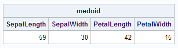
For these data, the 83rd row is the one that minimizes the sum of distances to all other points. The 4-dimensional coordinates of the points are shown in the output.

/* write to SAS data set for visualization. Include the sum of distances for each point */
sumDist = sumDist(X);
Y = sumDist || X;
create Out from Y[c=('sumDist' || varNames)];
   append from Y;
close;
create Out2 from medoid[c=('X1':'X4')];
   append from medoid;
close;
QUIT;
 
data All;
label sumDist = "Sum of Distances";
set Out Out2;
run;
 
ods graphics / width=480px height=480px;
title "Visualization of the Medoid in Fisher's Iris Data";
/* color palette from https://blogs.sas.com/content/iml/2016/07/18/color-markers-third-variable-sas.html */
%let attrs = markerattrs=(symbol=CircleFilled) transparency=0.25 colormodel=(CX3288BD CX99D594 CXE6F598 CXFEE08B CXFC8D59 CXD53E4F);
proc sgplot data=All aspect=1 ;
   scatter x=SepalLength y=SepalWidth / colorresponse=sumDist &attrs;
   scatter x=x1 y=x2 / markerattrs=(symbol=StarFilled size=10 color=black) legendlabel="medoid";
   xaxis grid;
   yaxis grid;
run;
 
proc sgplot data=All aspect=1 ;
   scatter x=PetalLength y=PetalWidth / colorresponse=sumDist &attrs;
   scatter x=x3 y=x4 / markerattrs=(symbol=StarFilled size=10 color=black) legendlabel="medoid";
   xaxis grid;
   yaxis grid;
run;

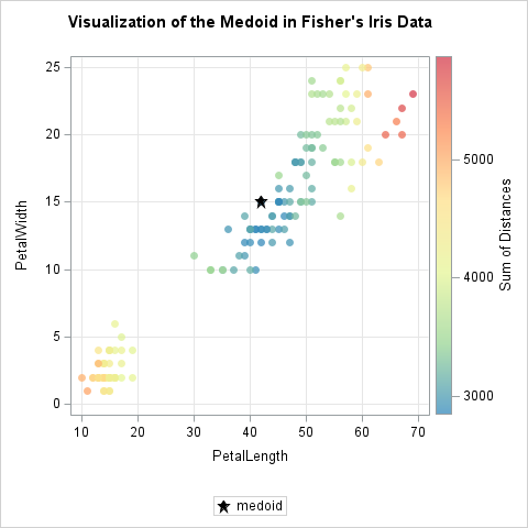
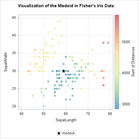
The scatter plots show that the medoid (marked with a star) is a data value that is near the "center" of the point cloud. resulting datasets to generate scatter plots of pairs of variables. The key insight is that even in 4-D, the medoid still represents the most centrally located, robust observation in the set.

Remarks on the medoid computation

• Choice of distance: By default, the DISTANCE function computes the Euclidean distance. You can use the L1 or "Manhattan" distance instead by adding "L1" as a second argument. In theory, you can use any metric function such as the cosine similarity or Mahalanobis distance.
• Robustness: The medoid algorithm tends to be robust to outliers. I added some extreme values to the Iris data and noticed that the medoid did not change for my experiments.
• Standardization: For the Iris data, all variables are measured on the same scale (millimeters). As is common for distance-based algorithms, if your data contains variables that have different measurements (age, length, weight, rates, etc.), then you must standardize the data first. If you don't, the distance doesn't really make sense, and the computation will be dominated by the variable with the largest variance.
• Memory: A drawback of this method is that it computes the full (n x n) matrix of pairwise distances. This limits the number of data points that you can process. For example, I've previously calculated the RAM required by a square matrix. Processing 16,000 points requires just under 2GB of memory. Processing 40,000 observations requires 12GB, which might be more than your SAS administrator permits. It is not practical to use the algorithm in this article to process 100,000 points, which would require allocating 75GB of RAM. Instead, you would need to process the data by using block matrices to compute the smallest sum of distances.

Summary

The medoid is a robust choice for the "center" of a multivariate point cloud. Unlike means, centroids, and geometric medians, the medoid is always a point in the data. Mathematically, it is the point for which the sum of the distances to the other points is the smallest. This article used the standard Euclidean formula to measure the distance between points, but you can substitute other distance metrics. The SAS IML language enables you to compute the medoid in a vectorized manner independent of the number of points or their dimension.